
Methods For Unambiguous Electrical Delay Measurements Using A Vector Network Analyzer

By Donald Vanderweit, Keysight Technologies, Inc.*
*Keysight Technologies Inc., formerly Agilent Technologies electronic measurement business
The “electrical delay” of a device may be simply defined as the time it takes an electrical signal to pass through it. It is expressed in units of time, and varies with the frequency of the signal and other factors.
Measuring the electrical delay of devices like filters, long cables, or delay lines can present many challenges. The most common technique for measuring electrical delay is a reflection-based measurement, such as Time-Domain Reflectometry (TDR). But reflection-based measurements are not always possible. The Device Under Test (DUT) may contain repeaters or other non-reciprocal elements that have a high loss in the return direction, and prevent a reflection measurement. In cases where both ends of the link are available for measurement and a “through” measurement such as S21 is possible, a Vector Network Analyzer (VNA) can be a very effective tool for measuring electrical delay.
One side effect of the S21 method is an ambiguity in the electrical delay measurement brought about by the finite number of points in the measurement sweep. For most DUTs, this ambiguity is not a factor, but for DUTs with electrical delays greater than 1us, such as long delay lines and free space links, special methods should be used to eliminate this ambiguity.
The S21 Method
In this method, a vector network analyzer is used to measure S21 of the DUT across a range of frequencies (S21 is the ratio of the voltage out of the DUT to the voltage in). A vector network analyzer tracks phase as well as magnitude. For a device with a non-zero electrical delay, the phase shift between the input and the output of the DUT will change due to the frequency of the signal. Lower frequency signals have a longer wavelength than higher frequency signals, and will go through fewer cycles passing through the DUT. Even for a perfectly linear DUT, the phase trace of S21 will have a slope that is related to the electrical delay.
By displaying the phase component of the S21 trace, we can observe the effect of the DUT on the signal at different frequencies and calculate the electrical delay. This is most easily done using an S21 trace, which is formatted to show the “unwrapped” phase of the trace. “Wrapped” phase data “wraps” around so that the data does not exceed +/- 180 degrees. By showing unwrapped phase, the network analyzer displays the trace data in a way that preserves long trends. A long increase or decrease in phase can be shown as passing through thousands of degrees.
For a device with an electrical delay that is constant over this frequency range, the trace will appear as a straight line (Figure 1). This line shows how the electrical delay of the DUT affects the phase differently at different frequencies.
The phase change caused by the device is itself a function of the period of the wave and the electrical delay (in time) of the device:
Delta phase = electrical delay (s)/period of the waveform (s/period) * 360 (degrees/period)
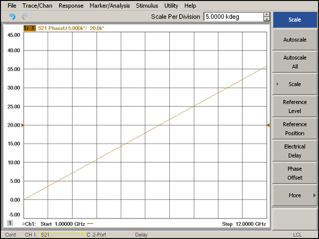
Figure 1: Display of Unwrapped Phase Trace for Delay Line
Since period = 1/frequency, the equation becomes:
Delta phase = electrical delay*frequency *360
From this equation, we see that lower frequencies go through less of a phase shift than higher frequencies and that the relationship between frequency and phase is a straight line (for an ideal delay line), where the slope of the line is given by:
Slope = electrical delay*360.
It would appear from this last relationship that it would be easy to determine electrical delay by measuring the slope of this line, or by adjusting the electrical delay setting (found in some VNAs) until the trace is horizontal (some VNAs even automate this process with a special marker or macro).Another common method is to display the trace using the “Delay” format. This format is intended to show group delay, which is the change in electrical delay expressed as a function of the change in frequency. If the device is linear, the trace will show a flat line where the value on the Y-axis is the electrical delay.
All of these methods rely on the same basic calculations. While they are very useful for electrically short devices, the finite spacing of the frequency points on the network analyzer can cause a false result, and lead to an ambiguity in the measurement.
Unwrapped Phase
The source of this ambiguity is the way that the VNA measures and displays phase. For example, consider a frequency sweep from 1 to 2 GHz, with 101 points. The frequency spacing (the difference between adjacent frequency measurement points) would be:
(2GHz – 1GHz)/(101-1) = 10MHz.
Consider the difference in phase between two adjacent points, after the signal has passed through the delay line. From our equation above, the phase difference between two adjacent points would be given by electrical delay * frequency spacing * 360. In our example, the frequency spacing is 10MHz. This suggests that for electrical delay greater than (1/10MHz) = 100ns, the phase change between adjacent points would be greater than 360 degrees. But, the algorithm the VNA uses to calculate phase does not account for phase changes greater than 360 degrees. Because measurements are made at discrete points, without knowledge of the signal in between, the VNA has no way of knowing how many phase revolutions the signal has passed through in travelling down the cable, and it cannot distinguish between a change of 10 degrees, 370 degrees, 730 degrees, etc. The value could be 10 degrees +/- n*360 degrees, where n is any integer.
In the ordinary “Phase” display, only values between -180 degrees and 180 degrees are selected for display. In the “Unwrapped Phase” display, the VNA examines trends in the signal to reproduce the long term trend. If the display is trending upward, the VNA will continue the trace upward by adding 360 degrees when the phase wraps around, or subtracting 360 degrees if the trace is trending downward.
The ambiguity between these multiples of 360 degrees causes an ambiguity in the electrical delay measurement. For our example, with frequency spacing of 10MHz, the slope would look the same for a delay line of 10ns, 110ns, 210ns, etc. The slope repeats every 100ns, or 1/(frequency spacing).
Removing the Ambiguity
For DUTs with a short electrical length, this presents no problem, but for longer DUTs, this ambiguity can force us to decide between several possible answers. Fortunately, armed with the equations above, we can increase the unambiguous measurement range until it is larger than the estimated electrical delay. There are a few ways to accomplish this:
- Reduce the spacing between frequency measurement points:
By adding more points to the trace, or reducing the span of the trace, the spacing between adjacent points can be reduced. This technique gives a direct benefit. Doubling the number of points in a trace (or reducing the span by a factor of 2) doubles the unambiguous measurement range. Taking this simple step may be enough to increase the unambiguous range beyond the estimated electrical delay of the DUT. Once the settings are adjusted, the electrical delay can be calculated from the slope of the trace using any of the methods described above.
This also leads to a handy method for verifying that the frequency spacing is small enough for the measurement. Change the number of measurement points without changing the frequency span of the trace. Try a few different settings for the number of points. If the slope of the trace does not change, the frequency spacing is sufficiently small.
For real-world DUTs the trace will not be exactly linear. This deviation from linearity is related to Group Delay, and is itself a very useful metric of the characteristics of the DUT. Finding the “correct” value for the electrical delay in these cases may be done with a linear curve fit of the data, or by using the trace statistics function included with many VNAs.
- Using segmented sweep:
In some extreme cases, reducing the span and/or increasing the number of points may not be enough. This could be true of very long delay lines (>10km), free-space links, etc. In these cases, the expected delays are very long, and it may be difficult or undesirable to reduce the frequency spacing to a point where this delay value falls in an unambiguous range. For example, a 10km optical delay line would have an electrical delay on the order of 50us. To increase the unambiguous range beyond this value, we would need to set the VNA trace with a frequency spacing of <20kHz. This can be done with 10,001 points and a span of <200MHz. This is certainly possible with most VNAs, but measurements across wider frequency ranges (or faster sweeps) may be desired. For these cases, we can take advantage of the “segmented sweep” feature found in many VNAs. As the name suggests, segmented sweep allows us to take measurements at segments of the frequency spectrum, skipping over the frequencies in between.
The real strength of this technique is that by using different frequency spacing in different segments, the unambiguous range of the segments will be different from each other. This effectively increases the unambiguous measurement range of the entire trace to the lowest common multiple of the two ranges. For example, suppose we set out to measure a device with an electrical delay of 1000ns. The insertion loss of the device is acceptably low in the range of 1 to 5 GHz.
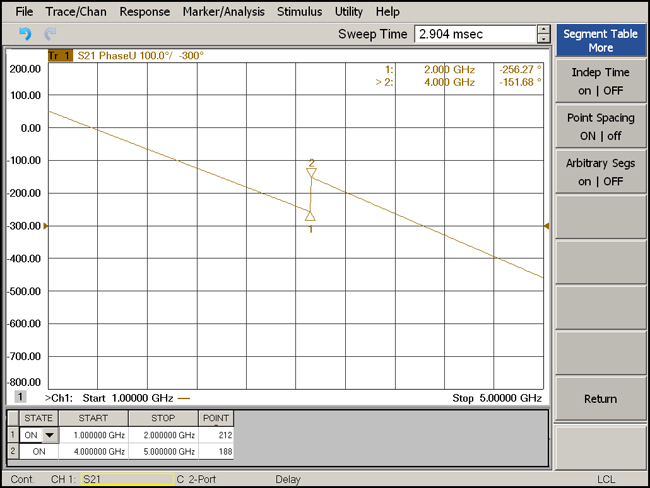
Figure 2: Screen shot of the VNA making a segmented sweep measurement
To maximize the unambiguous measurement range, we will set up a segmented sweep in which the two segments have frequency spacing values that are not related to each other through common factors:
Segment 1: Sweep from 1 to 2 GHz over 212 points (frequency spacing of about 4.74MHz)
Segment 2: Sweep from 4 to 5 GHz over 188 points (frequency spacing of about 5.35MHz)
The unambiguous range is 87ns for the first segment and 91ns for the second segment. For our 1000ns delay line, Segment 1 could yield a result of 789ns, 1000ns, or 1211ns (and other values +/- 211ns). Segment 2 would yield results of 812ns, 1000ns, or 1187ns. The unambiguous range of the two segments together would be 187*211ns, or 39457ns, which is well beyond our expected value, leaving 1000ns as the only choice common to the two segments.
This works very well in cases where the slopes of the segments are fairly constant. If the slopes of the lines are not particularly linear, using the linear curve fitting method with segmented sweep presents a challenge. The two segments should produce two different slopes. To determine the unambiguous value, the user would need to solve a Diophantine equation:
Delay = (1/slope 1) + m*(1/freq spacing 1) = (1/slope 2) + n*(1/freq spacing 2)
or
(1/slope 2) – (1/slope 1) = m*(1/freq spacing 1) - n*(1/freq spacing 2)
where m and n are integers. This can be difficult to solve if the error bars on the slope measurements are too high.
A crude but effective way to get around this would be to manually adjust the electrical delay setting on the VNA until both lines are horizontal. In practice this method is quite dramatic: it is easily apparent when the correct range is reached. The most dramatic effect occurs when the two segments are separated in frequency (that is, when the high value of the lower range and the low value of the higher range are not the same). In this case, the user can fine-tune the electrical delay until the lower range and upper range segments come together.
Using the S21 phase measurement capabilities of a vector network analyzer, even delay lines with high loss and very long electrical delays can be measured.
About The Author
 Donald Vanderweit, Application Engineer, Keysight Technologies, Inc.
Donald joined Keysight (then Agilent) Technologies in 2006. He is an application engineer supporting RF and microwave products in the Southern California region. His focus is within the Aerospace and Defense industries with special emphasis in the latest trends in radar, electronic warfare, telemetry, and military communications. Before joining Agilent, Donald worked in the broadcast and entertainment industries. He received his MSEE from the University of Colorado at Boulder in 1988.